Organization of the Manual
1. General Information
This section contains general information about the MPD experiment and the MpdRoot environment, including the purposes, points of contact, and acronyms and abbreviations.
1.1 The MPD experiment at the NICA project
1.2 Purposes of the MpdRoot framework
1.3 MpdRoot Coding Convention
1.4 Points of contact
2. Installation
The second section points to installation methods of the MpdRoot framework based on your particular needs.
2.1 Installation Methods
2.2 Short Introduction to JupyterLab
2.3 How to add External dependencies
2.4 How to use Git and Gitlab
2.5 How to add custom QA histogram
3. MpdRoot Structure
This section contains the information about the directory structure of the MpdRoot framework.
4. Simulation and Reconstruction Tasks
The fourth section details the simulation and reconstruction macros, their main parts, execution scheme. It lists possible event generators and transport packages which can be used in detector simulation. It contains information about macros to be run by ROOT environment and Analysis Tutorial.
4.1. Virtual Monte Carlo
4.2. Event generators
4.3. Simulation of the MPD experiment
4.4. MPD event reconstruction
4.5. Analysis Tutorial
5. Unified Database for MPD Offline Data Processing
The section describes the developed Unified Database designed as offline data storage of the MPD experiment. The scheme of the Unified Database and its parameters are briefly presented. In addition, C++ interface developed for the access to the database is concisely described (in progress).
6. Distributed Computing
The last section contains links to information describing the design approaches and methods of cluster development for storing and processing of data obtained at the MPD detector. The current cluster scheme and structure are presented; along with the software for building data storage and parallelization of the MPD data processing.
6.1. MPD dirac application
1. General Information
1.1 The MPD experiment at the NICA project
NICA Multi Purpose Detector
The MPD apparatus has been designed as a 4π spectrometer capable of detecting of charged hadrons, electrons and photons in heavy-ion collisions at high luminosity in the energy range of the NICA collider. To reach this goal, the detector will comprise a precise 3-D tracking system and a high-performance particle identification (PID) system based on the time-of-flight measurements and calorimetry. The basic design parameters has been determined by physics processes in nuclear collisions at NICA and by several technical constrains guided by a trade-of of efficient tracking and PID against a reasonable material budget. At the design luminosity, the event rate in the MPD interaction region is about 6 kHz; the total charged particle multiplicity exceeds 1000 in the most central Au+Au collisions at √sNN = 11 GeV . As the average transverse momentum of the particles produced in a collision at NICA energies is below 500 MeV/c, the detector design requires a very low material budget. The general layout of the MPD apparatus is shown in Fig. 1. The whole detector setup includes Central Detector (CD) covering ±2 units in pseudorapidity (η) .
The aim of this Project is to build a first stage of the MPD setup, which consists of the superconducting solenoid, Time-Projection Chamber (TPC), barrel Time-Of-Flight system (TOF), Electromagnetic Calorimeter (ECal), Zero-Degree Calorimeter (ZDC) and Fast Forward Detector (FFD).
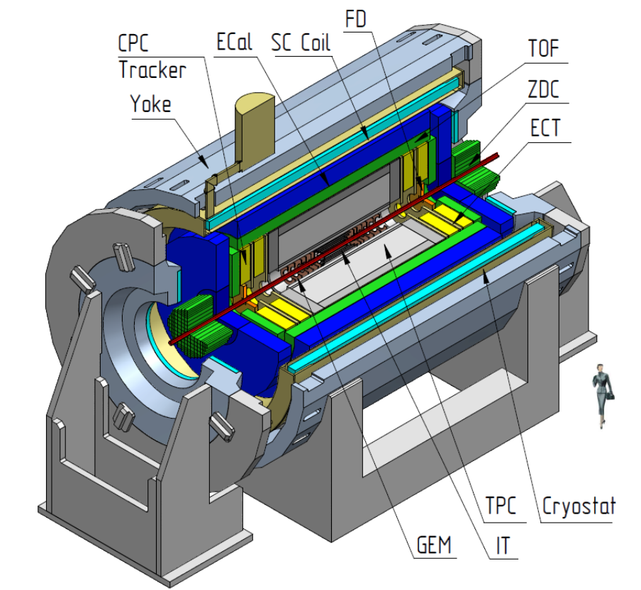
Figure 1: A general view of the MPD detector with end doors retracted for access to the inner detector components. The detector consist of three major parts: CD-central detector, and (FS-A, FS-B) – two forward spectrometers (optional). The following subsystems are drawn: superconductor solenoid (SC Coil) and magnet yoke, inner detector (IT), straw-tube tracker (ECT), time-projection chamber (TPC), time-of-flight system (TOF), electromagnetic calorimeter (EMC), fast forward detectors (FFD), and zero degree calorimeter (ZDC).
1.2 Purposes of the MpdRoot framework
The software and computing parts of the MPD project is responsible for the activities including design, evaluation and calibration of the detector; storing, access, reconstruction and analysis of the data; and development and maintenance of a distributed computing infrastructure for physicists engaged in these tasks. To support the MPD experiment, the software framework MpdRoot is developed. It provides a powerful tool for detector performance studies, event simulation, and development of algorithms for reconstruction and physics analysis of data of the events registered by the MPD experiment. The MpdRoot is based on the ROOT environment and the FairRoot framework developed for the FAIR experiments at GSI Institute.
The flexibility of the framework is gained through its modularity. The physics and detector parts could be written by different groups. In the applied framework, the detector response simulated by a package currently based on the Virtual Monte Carlo concept allows switching code. For a realistic simulation of various physics processes, an interface to the event generators for nuclear collisions, e.g. UrQMD, Pythia and FastMC, is provided. One can easily choose between different modules, e.g.event generators. The same framework – MpdRoot is used to define the experimental setup, provides simulation, reconstruction, and physics analysis of simulated and experimental data. Using the same internal structure the user can compare easily at any time the real data with the simulation results.
The MpdRoot environment also includes the tool for event navigation, inspection and visualization. The MPD event display for Monte-Carlo and experimental data is based on the EVE (Event Visualization Environment) package of the ROOT. The event display macro can be used to display both Monte-Carlo points and tracks, and reconstructed hits and tracks, together with the MPD detector geometry. The Event Manager implemented in the framework delivers an easy way to navigate through the event tree and to make cuts on energy, particle PDG codes, etc. in selected events.
1.3 MpdRoot Coding Convention
Please follow the link to read.
2. Installation
OS support
MpdRoot runs natively on Linux.
If you are not using Linux, you can run it in virtual machine:
– use VMware Workstation Player to install Linux in Windows
– use VMware Fusion Player to install Linux in Mac
We recommend to use any Red Hat based Linux distribution: AlmaLinux, Rocky Linux, Fedora, …
2.1 Installation methods
1. On the cluster
2. Locally using CVMFS (recommended)
3. Locally using aliBuild (for advanced users)
2.2 JupyterLab
This is an introduction to JupyterLab use.
Note: this tutorial works for user and developer MpdRoot installations
Useful commands:
toolbox enter a9-nica-dev
wget -N https://git.jinr.ru/nica/nicadist/-/raw/master/scripts/jupyter-fix.sh
chmod +x jupyter-fix.sh && ./jupyter-fix.sh
2.3 External dependencies
MpdRoot does have additional support for external packages required by some of the MpdRoot developers for the future versions of code, but are not part of the main branch yet. We don’t add these packages as compulsory dependencies, until the code requiring them does not land in the main branch. This allows enough flexibility during the development process without clogging the code with dependencies, that may not be even needed in the future.
To compile MpdRoot with externally supported package (say, Eigen 3), first load its module with mpddev, i.e. instead of line “module add mpddev” in Installation Page write:
module add mpddev Eigen3Include and library directories of supported external packages are added to BASE_INCLUDE_DIR and BASE_LIBRARY_DIR. Please note, that after loading module, variables moduleName_ROOT are created automatically.
Currently supported external packages:
| Package | Module name | Variable MpdRoot looks for | Variables available in CMake | |
|---|---|---|---|---|
| Eigen3 | Eigen3 | EIGEN3_ROOT | Eigen3_INCLUDE_DIRS, EIGEN3_ROOT | |
| FFTW | FFTW | FFTW_ROOT | FFTW_INCLUDE_DIR, FFTW_LIBDIR, FFTW_ROOT | |
| mxpfit | mxpfit | MXPFIT_ROOT | MXPFIT_INCLUDE_DIR, MXPFIT_ROOT | Eigen3, fftw |
Note: dependencies are auto-loaded, i.e. it is enough to call
module add mxpfit2.4 How to use Git and Gitlab
This is quick tutorial on how to use capabilities of GIT tools for software development in team.
You can download repository zip archive without registration and SSH keys (only for read) here: MpdRoot archive.
1. To access the Git repository
- Register on the JINR GitLab site with @jinr.ru mail.
- Add SSH key in your personal Gitlab profile!
- Add your Git username and set your email
It is important to configure your Git username and email address, since every Git commit will use this information to identify you as the author.
On your shell, type the following command to add your username:
git config --global user.name "YOUR_USERNAME"To set your email address, type the following command:
git config --global user.email "your_email_address@example.com"To view the information that you entered, along with other global options, type:
git config --global --list2. To get a Git repository use this command
git clone git@git.jinr.ru:nica/mpdroot.git3. To download the latest changes in the project
git pull4. To view all branches in the project
git branch -r5. To work on an existing branch
git checkout NAME-OF-BRANCH6. To create a new branch and start working with it
Please use names for branches in accordance with the task for common understanding, like: feature-new-geometry or bugfix-old-problem. Spaces won’t be recognized in the branch name, so you will need to use a hyphen or underscore.
git checkout -b NAME-OF-BRANCH7. To add new file or folder in your branch
git add NAME-OF-FILE8. To add all new files or folders in your branch
git add .9. To view the changes you’ve made
It’s important to be aware of what’s happening and the status of your changes. When you add, change, or delete files/folders, Git knows about it. To check the status of your changes:
git status10. View differences
To view the differences between your local, unstaged changes and the repository versions that you cloned or pulled, type:
git diff11. To save all changes that you made in local machine Git repository
git commit -am "Some comments add here"12. To save the changes in remote server machine Git repository (origin branch)
git push origin NAME-OF-BRANCH13. To merge
If you want merge NAME-OF-BRANCH with protected dev branch create merge request on GitLab site for MpdRoot. Then if your branch has passed the testing without errors and approval of CodeOwners, your code might be merged.
If something went wrong
14. Delete all changes in the local Git repository
To delete all local changes in the repository that have not been added to the staging area, and leave unstaged files/folders, type:
git checkout .15. Unstage all changes that have been added to the staging area
To undo the most recent add, but not committed, files/folders:
git reset .Useful links
- GIT software for Windows download here: Tortoise git client (for example)
- Full Git Documentation: http://git-scm.com/book/ru/v1
- How To use GIT: http://githowto.com/ru
2.5 Adding custom QA histograms
IMPORTANT: This feature works for mpddev versions >= v24.06.24. Do a complete rebuild (rm -rf /mpdroot/build) before using it for the first time.
You have a task you are using in your macro
class MyOwnTask : public FairTask {...}Your goals are
1. Adding your own histograms, which you can update during each event
2. View those histograms in a .root file after the run finishes
Do:
1. In the constructor of MyOwnTask create your histograms, and add them to fTaskHistograms
MyOwnTask::MyOwnTask(){
 TH1F* histo_1d = new TH1F("1D","1D_title",100,-4,4);
 fTaskHistograms->Add(histo_1d);
 TH2F* histo_2d = new TH2F("2D","2D_title",100,0.,10.,100,0.,10.);
 fTaskHistograms->Add(histo_2d);
}
You can then fill and update your histograms anytime during your run.
2. At the end of the run, your histograms are written into file TasksHistograms.root, which you can view in TBrowser.
– each task has its own directory with all of the task histograms
– task directories are ordered and named after MyOwnTask::GetName()
Simple exercise:
Add the code in red into digitizer’s constructor, and check the generated TasksHistograms.root file
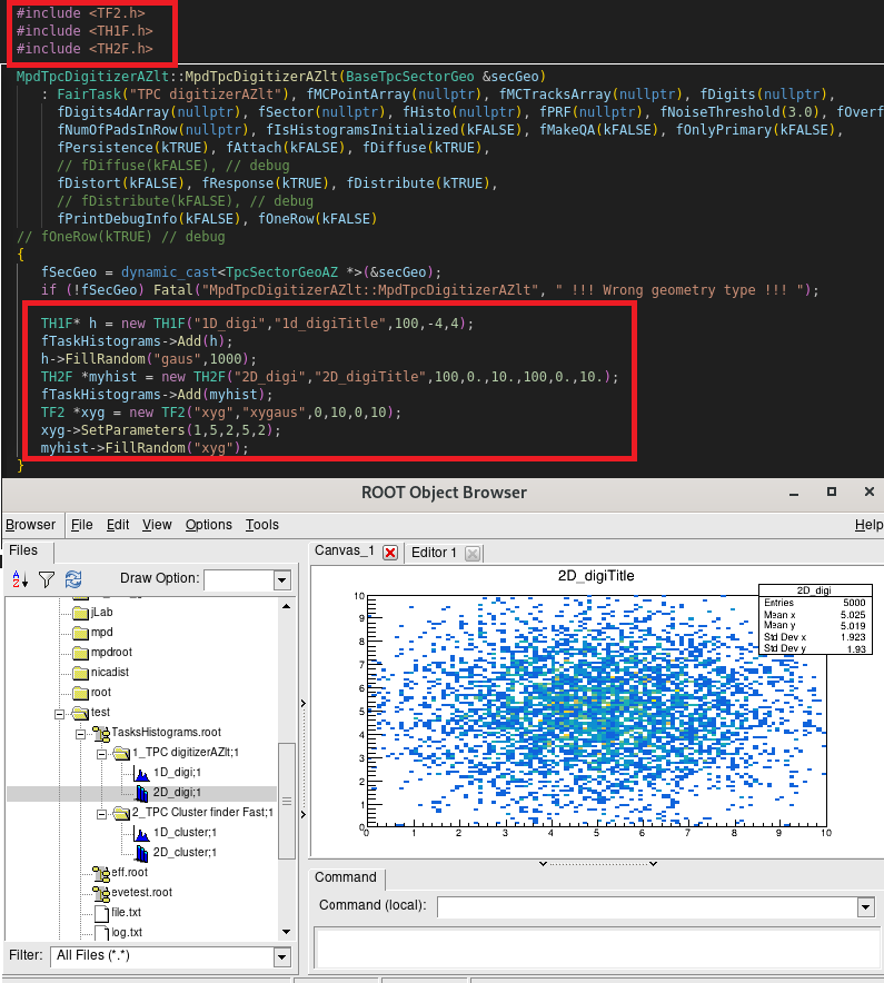
For your convenience, the selected chunks of code for copy/paste-ing:
#include <TH1F.h>
#include <TH2F.h>
#include <TF2.h>

TH1F* h = new TH1F("1D_digi","1d_digiTitle",100,-4,4);
fTaskHistograms->Add(h);
h->FillRandom("gaus",1000);
TH2F *myhist = new TH2F("2D_digi","2D_digiTitle",100,0.,10.,100,0.,10.);
fTaskHistograms->Add(myhist);
TF2 *xyg = new TF2("xyg","xygaus",0,10,0,10);
xyg->SetParameters(1,5,2,5,2);
myhist->FillRandom("xyg");
3. MpdRoot Directories
cmake – CMake scripts to compile the MpdRoot software, CMake generates native Makefiles for all supported platforms
core – contains MPD core classes (to be updated)
- mpdBase – base classes of MPD environment such as MpdEvent, MpdVertec, MpdHelix, MpdTrack
- mpdDst
- mpdField – classes to work with magnetic fields
- mpdPassive
- mpdPid
detectors – contains classes of detectors present in MPD, each with its own subdirectory (to be updated)
- bbc
- bmd
- emc
- etof
- ffd
- mcord
- sts
- tof
- tpc
- zdc
gconfig – macros with cuts and settings of particle transport packages (Geant,Fluka…) for event simulation
geometry – files with geometries of the MPD subdetectors in ROOT (.root) or ASCII (.geo) formats
input – text files with different MPD parameters and detector mappings
macro – ROOT macros for simulation, reconstruction and physical analysis tasks (to be refactored).
macros – refactored ROOT macros for simulation, reconstruction and physical analysis tasks.
physics – (to be updated)
reconstruction – ROOT macros for simulation, reconstruction and physical analysis tasks (to be updated)
- kalman – Kalman filter classes to reconstruct particle tracks
- lheTrack
scripts – system scripts
simulation – classes used in MC simulation
- generators – classes of the event generators: UrQMD, Box, Pluto, etc.
- mcDst
- mcStack
tools – various tools used mainly to develop MPDroot framework
- database – C++ database interface for getting data of the MPD experiment
- documentation – files to generate doxygen and reference manual
- eventDisplay – classes for visualization and monitoring of collision events and detector geometries
- tdd – test driven development toolkit
4. Simulation and Reconstruction Tasks
4.1. Virtual Monte Carlo
Basically, there are two ways to simulate the behavior of a system: either one can describe its evolution analytically, in which case computers are used to find the solution of the dynamic equations, or a probabilistic approach is used, in which at each step pseudo-random numbers are used to select one among different physics processes. Example of the first approach is the computation of charged particle paths inside a magnetic field. When dealing with the interactions of particles with matter, the second approach is usually followed, because of the variety of possible physics processes and of their discrete nature. Because such approach is based on pseudo-random numbers, it is usually called a “Monte Carlo” method.
TVirtualMC class of the ROOT environment provides a virtual interface to Monte Carlo applications, allowing the user to build a simulation independent of any actual underlying MonteCarlo implementation itself. A user will have to implement a class derived from the abstract Monte Carlo application class. The concrete Monte Carlo implementation such as Geant3, Geant4, Fluka, is selected at run time–when processing a ROOT macro where the concrete Monte Carlo object is instantiated. This allows for comparison between different engines (necessary to estimate the theoretical uncertainties) using a single application. The concept of Virtual MonteCarlo has been developed by the ALICE Software Project.
Monte Carlo simulations always have to describe the input particles, together with their interactions, and the detector (geometry, materials and read-out electronics). The definition of particles, available interactions and detector is carried on during the initialization phase. The main body of the application is then a loop over all particles that are traced through all materials until they exit, stop or disappear (by decay or annihilation). The tracing is done in a discrete fashion: at each step, the detector volume is found in which the particle is located and pseudo-random numbers are used to “draw” one among possibly several physical processes, to simulate the interaction of the particle with the matter. If an interaction occurs, the energy lost by the particle is computed and subtracted from its kinetic energy. When the latter reaches zero, the particle stops in such volume, other wise a new step is performed.
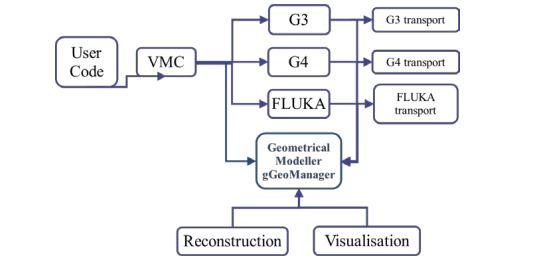
Figure 2: Geometrical Modeller (gGeoManager) for the MC simulation and subsequent use in reconstruction and visualization
Having computed the energy lost by all particles inside the detector, one has to simulate the behavior of the read-out electronics. This is usually done later, with another program that receives the energy lost in different locations as input, but it can also be done by the very same application that is performing the particle tracing inside the detector. Usually, the simulation of the read-out electronics also involves some use of pseudo-random generators, at least to simulate the finite resolution of any real measuring device.
The Virtual Monte Carlo (VMC) allows to run different simulation Monte Carlo without changing the user code and therefore the input and output format as well as the geometry and detector response definition. It provides a set of interfaces, which completely decouple the dependencies between the user code and the concrete Monte Carlo. The implementation of the TVirtualMC interface is provided for two Monte Carlo transport codes, GEANT3 and GEANT4. The implementation for the third Monte Carlo transport code, FLUKA, has been discontinued.
The VMC is now fully integrated with the ROOT geometry package TGeo, and users can easily define their VMC application with TGeo geometry definition.
4.2. Event generators
Event generators are software libraries that randomly generate high-energy particle physics events. MonteCarlo (because they exploit Monte Carlo methods) event generators are essential components of experimental analyses today and are also widely used by theorists and experiments to compare of experimental results with theoretical predictions and to make predictions and preparations for future experiments.
Monte Carlo generators allow to include theoretical models, phase space integration in multiple dimensions, inclusion of detector effects, and efficiency and acceptance determination for new physics processes. All event generators split the simulation up into a set of phases, such as initial-state composition and substructure, the hard process, parton shower, resonance decays, multiple scattering, hadronization and further decay. As a result, event generator produces the final-state particles, which feed into the detector simulation, allowing a precise prediction and verification for the entire experimental setup.
The MpdRoot framework supports an extended set of event generators (physics models) for particle collisions, which are commonly used in HEP experiments, such as:
• Ultrarelativistic Quantum Molecular Dynamics (UrQMD)
• Quark Gluon String Model (QGSM, LAQGSM)
• Shield
• Parton Hadron String Dynamics (PHSD, HSD)
• Pluto
• Hybrid UrQMD
• EPOS
• 3 Fluid Dynamics (for baryon stopping)
The Figure 3 shows the place of the event generators in the data processing chain and the further steps of simulation in particle physics.
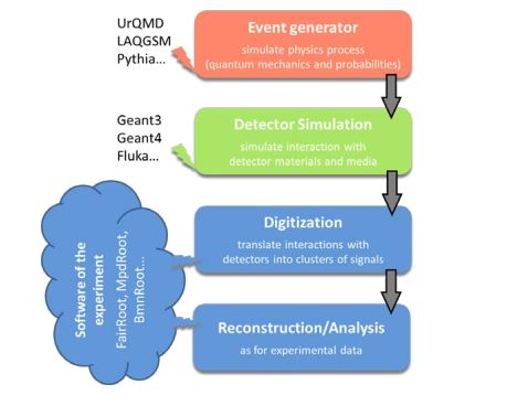
Figure 3. Simulation and analysis steps of high energy physics experiment
Partly due to historic reasons, many event generators are written in Fortran, newer ones are usually implemented in C++ language. Most particle collision (event) generators produce files of own format, which is then used in simulation of the experiment. The Figure 4 presents the steps above with file storage levels of the MpdRoot in more details.
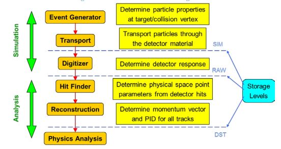
Figure 4. Data processing steps and storage levels of the MPD experiment
4.3. Simulation of the MPD Experiment
MPD simulation includes interactions and particles of interest, geometry of the system, materials used, generation of test events of particles, interactions of particles with matter and electromagnetic fields, response to detectors, records of energies and tracks, analysis of the full simulation at different detail and visualization of the detector system and collision events. As the events are processed via the simulation, the information is disintegrated and reduced to that generated by particles when crossing a detector.
Simulation in high energy physics experiments uses transport packages to move the particles through experimental setup from initial state or origin files produced by event generators, such as UrQMD or QGSM described above. Geant (short from “geometry and tracking”) transport package is developed at CERN and most commonly used today. Geant3 was implemented in Fortran programming language whereas Geant4 is developed in C++.
Transport includes detailed description of detector geometries and propagates all particle tracks through detector materials and media. The detector geometries are described by Geant3/Geant4 native geometrical models. During tracking of all particles through detectors, Geant forms the detector responses (hits) which are used in reconstruction task. In order to evaluate the software and detector performance, simulated events are processed through the whole cycle and finally the reconstructed information about particles is compared with the information taken directly from the Monte Carlo generation.
To simulate MPD events of particle collisions with a fixed target, runMC macro is used. The main macro lines are described below.
Initially, all libraries required for simulation and geometries are included by:
#include "commonFunctions.C"
#include "geometry_stage1.C"
It parses media definition and creates passive volumes, such as cave, pipe, magnet, cradle, and subdetectors: FFD, TPC, TOF, EMC, ZDC, MCORD.
Function parameters of the main body of the macro:
EGenerators generator - used generator, default value BOX
EVMCType vmc - used VMC, default value Geant3
Int_t nStartSeed - initial seed number
TString inFile – path of the input file with generator data if required;
TString outFile – path of the result file with MC data, default value: evetest.root;
Int_t nStartEvent – number (start with zero) of the first event to process, default: 0;
Int_t nEvents – number of events to transport (0–all events in the input file), default: 2;
Bool_tflag_store_FairRadLenPoint – whether to enable estimate radiation length data, default: kFALSE;
Int_t FieldSwitcher - 0 corresponds to the constant field (default), 1 corresponds to the field map stored in the file (default).
Then in the main body of runMC.C macro the simulation run is initialized along with initialization of geometry and the event generator is defined, which will be used to simulate MPD events.
FairRunSim* fRun = new FairRunSim();
geometry_stage1(fRun);

FairPrimaryGenerator* primGen = new FairPrimaryGenerator();
fRun->SetGenerator(primGen);
One can choose and tune one of the following event generators: BOX, FLUID, HSD, ION, LAQGSM, MCDST, PART, SMASH, UNIGEN, URQMD, VHLLE.
To select event generator, Add Generator function of FairPrimaryGenerator class is used.
Files of different event generators are located on the NICA cluster. If you do not have access to the cluster, you can use, for example, a simple particle BOX generator (default) to propagate selected particles to the desired directions. BOX generator is used without any input files for the simulation macro.
In the next step, the output file name is specified:
fRun->SetOutputFile(outFile.Data());The magnetic field set by map (ASCII or ROOT) file or constant field is chosen in the next lines of the macro. In the MPD experiment the transition from a constant magnetic field to real field map, interpolation of the field between map nodes and extrapolation of the field map to out-of-magnet region were made.
The following line enables or disables radiation length manager:
fRun->SetRadLenRegister (flag_store_FairRadLenPoint);The manager determines the particle fluency through a certain boundary (surface) and deduces a map. Knowing the volume and density of the object of interest and the specific energy loss, dose scan be estimated. Therefore, FairRadLenManager class estimates radiation length data and can answer the questions: “What energy dose will be accumulated during a certain time of operation?” and “How to create physical volumes with correct material assignment?”.
The next function initializes MPD simulation, i.e. Virtual Monte Carlo classes and tasks (if they are used in simulation): fRun->Init(). To run event simulation, the following line is executed: fRun->Run(nEvents). The Figure 5 presents the main modules of the MpdRoot framework and their relationship during the simulation.
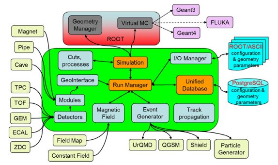
Figure 5: The scheme of the MpdRoot modules in the simulation
Input/Output manager (shown on the figure as I/O manager) called the Runtime Parameter Manager is the manager class for all parameter containers and based on ROOT TFolder and TTree classes. The Runtime Manager includes container factory, list of parameter containers and list of runs. The parameters are stored in the containers, which are created in the Init() function of the tasks via the container factory or produced from ASCII or ROOT files in the macro.
Subdetector geometries can be defined using different input formats: ASCII or ROOT files (Root Geometry format presented in the form of TGeoVolumes tree) or defined directly in the source code. The ASCII input format for detector geometry consists of volumes defined by the following sequence:
| Example | |
|---|---|
| Volume name | target |
| Mother volume name | pipe_vac_1 |
| Shape name | TUBE |
| Medium name | Gold |
| Shape parameters | 0. 0. -0.25 0. 2.5 0. 0. 0.25 |
| Positioning of the volume in a mother node: position and rotation matrix | 0. 0. 0. 1. 0. 0. 0. 1. 0. 0. 0. 1. |
The simulation result is evetest.root (default name) file with Monte Carlo data such as simulated track points and particle tracks in the MPD detector. It also includes MPD detector geometry stored in the FairBaseParSet container and presented by ROOT geometry manager (TGeoManager class) – its global pointer gGeoManager.
4.4. MPD Event Reconstruction
Event reconstruction is the process of interpreting the electronic signals produced by the detector to determine the original particles that passed through, their momenta, directions, and the primary vertex of the event. Event reconstruction consists of the following main steps:
• Hit reconstruction in subdetectors;
• Track reconstruction usually composed of: Searching for track candidates in main tracker; Track propagation, e.g. using Kalman filter; Matching with other detectors (global tracking)
• Vertex finding;
• Particle identification
The tasks for charged-track reconstruction in experimental high energy physics are pattern recognition (i.e. track finding) and track fitting. The common approach to the track reconstruction problem is based on the Kalman filtering technique. The Kalman filtering method provides a mean to do pattern recognition and track fitting simultaneously. The multiple scattering can also be handled properly by the method. The Kalman filter is a set of mathematical equations that provides an efficient computational (recursive) solution of the least-squares method.
The algorithm starts from track candidates (“seeds”), for which vectors of initial parameters and covariance matrices are evaluated. Then each track is propagated to some surface (detector or intermediate point). The new covariance matrix can be obtained using the Jacobian matrix of the transformation, i.e. the matrix of derivatives of propagated track parameters with respect to current parameters.
Tracks are usually defined by specifying their integer identification number, the particle code (integer code also known as the “PDG code” from the Particle Data Group maintaining a standard for designating Standard Model particles and resonances), the parent track (if any), and a particle object. In addition, each track has a (possibly empty) list of daughters that are secondary tracks originating from it. Precise knowing of the primary events vertex position essentially improves the momentum resolution and secondary vertices finding efficiency. The primary vertex is found by extrapolating all primary tracks reconstructed back to the origin, and its resolution is found as the RMS of the distribution of the primary tracks extrapolation at the origin. The global average of this distribution is the vertex position. The Figure 6 shows the place of event reconstruction in the processing chain for experimental and simulated data.
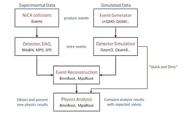
Figure 6: The chain of event processing for experimental and simulated data. To reconstruct MPD events of particle collisions with a fixed target registered by the MPD facility, runReco.C macro is used. Function parameters of the macro: TString inFile–path of the input file with MC data, default value: evetest.root; TString outFile–path of the result file with reconstructed DSTdata, default: mpddst.root; Int_t n StartEvent–number (start with zero) of the first event to process, default: 0; Int_t nEvents–number of events to process(0-all events of given file), default:10.
The main macro lines are described below. On the first steps the macro loading all libraries required for the reconstruction is included:
#include "commonFunctions.C"Then there construction macro creates FairRunAna (run analysis) class. To set input file with simulated or experimental data and output file with reconstructed data in DST format, the following lines are executed:
FairSource *fFileSource = new FairFileSource(inFile);
fRun->SetSource(fFileSource);
fRun->SetOutputFile(outFile);
The data reconstruction and analysis in the MpdRoot is organized by a list of analysis tasks (tasks can also be used in the simulation with FairRunSim class). Each task participating in event processing is inherited from the base class FairTask (TTask). Two main functions of tasks can be noted. Init() function initializes task and its variables and is executed inside FairRunAna::Init function. Exec(Option_t* option) function contains the main function code of the task and is called by FairRunAna::Run function. The scheme of task initialization and execution is presented on the Figure 7.
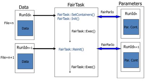
Figure 7. The scheme of task initialization and execution
The following example demonstrates task definition and adding to the task list in runReco.C macro:
MpdClusterFinderMlem* tpcClusFind = new MpdClusterFinderMlem();
fRun->AddTask(tpcClusFind);
In general, a task can be added not only to the FairRunAna instance but also to another task, i.e. all tasks can be organized into a hierarchy. If you want to get detector geometry from the given input file in your analysis task (if gGeoManager has not been known yet), you can execute:
FairRuntimeDb* rtdb = fRun->GetRuntimeDb();
FairBaseParSet* baseParSet=(FairBaseParSet*) rtdb->getContainer("FairBaseParSet");
and then use gGeoManager.
The Figure 8 presents the main modules of the MpdRoot framework and their relationship during the reconstruction.

Figure 8. The scheme of the MpdRoot modules in the reconstruction
The result DST file contains reconstructed (physical and geometrical) data about particles and particle tracks of collision events registered by the MPD facility.
4.5. Analysis Tutorial
In this repository you will find some macros to perform analysis within MpdRoot framework for the MPD (Multi-Purpose Detector) experiment at the NICA (Nuclotron-based Ion Collider fAcility) project.
Introduction
After run macros runMC.C and runReco.C from MpdRoot framework we can get two types of files: mpddst.root and mpddst.MiniDst.root which contains the required information of reconstructed particles to do analysis. In the following sections we will describe the basics of this, the macros available and explanations of how to use them.
The available outputs are:
• mpddst files. The mpdsim Tree contains the different branches: EventHeader, TpcKalmanTrack, Vertex, FfdHit, TOFHit, TOFMatching, ZdcDigi, MCEventHeader, MCTrack, MPDEvent.
• minidst files. The MiniDst Tree contains the different branches: Event, Track, BTofHit, BTofPidTraits, BECalCluster, TrackCovMatrix, FHCalHit, McEvent, McTrack.
Start with a Simple macro to Read Files
This kind of macros can be used with both, the user and developer installation of MpdRoot.
• Read mpdst files
• Read minidst files
Create a simple Task
To implement this tasks, we need the MpdRoot developer version, to add the classes and compile it.
• For mpddst files
• For minidst files
Compile MpdRoot with your analysis class
We need to create a folder in mpdroot with our class and the CMakeList.txt and LinkDef.h files to tell which classes should be added to the dictionary.
Macro to run the analysis with your class
This will allows you to implement your task and add several analysis task at the same time. The structure differs for mpddst files with respect to minidst files
Links
| Description | Repository |
|---|---|
| The Principal page of software | MpdRoot |
| Macros for simulation and transport | common |
| Macros for physical analysis | mpd |
| Centrality determination | CentralityFramework |
| ECAL Tutorial | ECAL new Geometry |
| Event Plane with ZDC | – |
| Directed and elliptic Flow | Flow |
5. Unified Database for MPD Offline Data Processing
MPD MC Events DB
Information about MPD Monte-Carlo data
MC Production Requests
Here you can write your request
MPD Alignment
Alignment Templates
MPD LogBook
ECAL DB
ECAL Technical Database
6. Mass Production & Distributed Computing
6.1. MPD dirac application
For efficient data processing of the MPD experiment, a heterogeneous, geographically distributed computing environment is currently being created on top of the DIRAC Interware. By 2019, standard workflow tests related to general Monte-Carlo generation were successfully carried out, which proved the possibility of using DIRAC for real scientific computation. At first, only Tier1 and Tier2 were used for that work, but later the “Govorun” supercomputer and the VBLHEP cluster were integrated into the system. The JINR EOS storage system is integrated and accessed via root protocol. Authentication is based on x509 certificates, and authorization is regulated by both DIRAC and VOMS.
At the moment, the heterogeneous, geographically distributed computing environment includes the Tier1 and Tier2 grid sites, the “Govorun” supercomputer, the cloud component of the MIСC JINR, the computing clusters of VBLHEP JINR and UNAM Mexico. The extensive use of different distributed resources made it possible to successfully complete more than 1000000 computing jobs. Each job was running approximately 6-7 hours. Request for all these jobs came from four MPD Physics Working Groups. They form requests with all the information relevant for data production in a special information system. The production manager uses this information to form job descriptions and submit them to DIRAC. Each job consists of two parts: Job Description information and Shell script that is executed on the worknode.
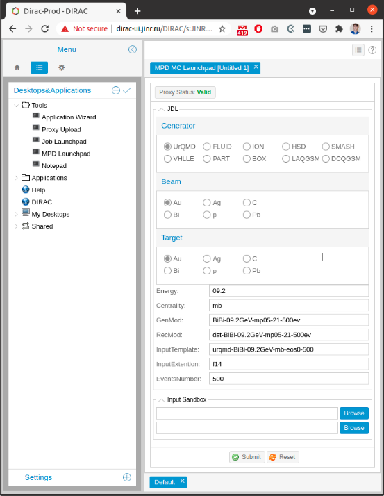
To simplify the process of job submission special web application was developed and integrated into the DIRAC web interface which is usually used for small workload submission, job monitoring, accounting check, and some other activities. With developed application user should just fill in all the physics parameters, define the number of collision events to be generated, and attach two files with the root code: run.mc and reco.mc. These files are written by physicists and contain the code related to the process of generation and reconstruction correspondingly.
Instructions
Users have to pass several steps in order to use the application.
1. Request user certificate on https://ca.grid.kiae.ru/RDIG/requests/new-user-cert.html
2. When the certificate is ready, it has to be loaded in the browser. That requires converting the certificate from pem format to p12 format.
3. Register in MPD Virtual Organization(VO) on the web-site:
https://lcgvoms01.jinr.ru:8443/voms/mpd.nica.jinr/user/home.action
4. Write to the responsible person from MPD to add user certificate to DIRAC system.
5. After confirmation, it is possible to access https://dirac-ui.jinr.ru
On the website, MPD application is placed in Tools -> MPD Launchpad.
In the MPD Launchpad user chooses all required options and provides parameters for the production. It is necessary to attach two scripts: runMC.C and reco.C. After that click on the button Submit.
The application is continuously developed and improved.